Merge sort

Background

Merge sort belongs to the group of "divide and conquer" algorithms. It is very efficient(runs in O(n * log₂n)) and makes low number of comparisons. One disadvantage is the amount of extra space that it requires. Normally this sorting is stable, meaning that it preserves the order of equal elements. The basic implementation is not adaptive, but adaptation could be added. We will discuss if and when that is necessary and good.

Advertise on this site. I promise you will like the rates :)

Divide and conquer

In programming, "Divide and conquer" is the principle of dividing a complex problem to sub-problems. The sub-problems are then divided to even simpler problems. This process continues until the problem is automatically solved or its solution is trivial. This leads to some of the most efficient algorithms that are used today.

The idea of merge sort

So we want to sort an array and we have the divide and conquer idea. Here is how it is applied in this case:

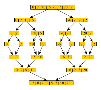
1. We take the array and split it in half. Then we repeat the same with each half until each half is of size 1 or 0. This is done through a recursion, but we will talk about that a little later.
2. An array of size 1 is trivially sorted.
3. The rest is a simple routine of combing two sorted arrays into one bigger. We continue to combine, until we combine all elements and our array is sorted.

That's it. It is that simple, yet super fast. As always, of course, we will visualize the idea for better understanding.

The merge routine

Dividing the array in two sub-arrays is a trivial task, so we will not go much into details there. The merging is where the actual work is done. It takes two arrays and combines them in the most efficient way.

The first key point is that the two arrays must be sorted before they are combined. The first time this procedure is called is with the arrays of size 1 and we know that a single element is always sorted. After that the arrays to be combined are already sorted, because they are merged into sorted arrays by the same function.

Let's take a look how the merging is done.
For the example we have the two arrays named "left" and "right".

    left = 0, 2, 5, 10
    right = -6, 2, 7, 20

We create two variables that point the current position in "left" and "right";

    leftIndex = 0;
    rightIndex = 0;

Now we can compare the values behind the two indices and take the smaller value.
In this case -6 is smaller so we take that value and write it in the result array.

result[0] = -6.

Once we took the value of -6 from "right", it is time to move the right index to the next number:

    rightIndex++;

We continue with the next pair of numbers from left and right. In this case the value in "left" is smaller, so:

    result[1] = 0;
    leftIndex++;

These steps will continue until all the numbers are filled in the "result" array.
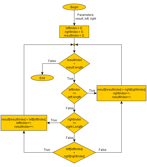
Here is a flow chart for the merging:

Merge sort

Merge sort is a recursive algorithm. As we said earlier it divides the array recursively until all sub-arrays are of size 1 or 0. Then it merges them by pairs into small sorted arrays and continues the process until all sub arrays are merged into one sorted array.

If you don't know what a recursion is this might seem really confusing. Recursion is a function which calls itself. Every recursion must have a base case which interrupts the calls and returns a result for the previous call. In our case the base is when the sub arrays are small enough so that they are trivially sorted(size 1 or 0).

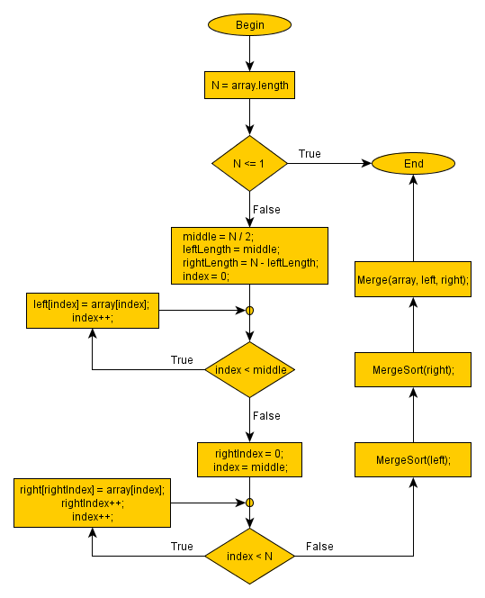
The flow chart below describes the procedure. You can see that it consists of several major parts:

1. Divide the array in two sub arrays - left and right
2. Make a recursive call for the left array
3. Make a recursive call for the right array
4. Merge the arrays.

Space complexity analysis

You probably noticed that the speed of this algorithm comes at the price of the extra space taken. This is the space that we need to create the extra left and right arrays. Since they are half the size of the original array, we will need 2 * N/2 extra space.

Also it uses several index variables to work with these arrays. Note that when we work with large arrays these will be insignificant. In other words merge sort uses N extra space for the left and right. This is a lot, compared to most of its rivals. For that reason people invented implementations that use N/2 or even in-place O(1) extra space. Anyway, the in-place version worsens the time complexity and it is not used much in practice.

Time complexity analysis

This analysis is more complex and need some visualization. Consider the first picture above where we sorted the array with 8 elements. The upper half of the graph only splits the array. Note that the actual work is done in the merging routine. It is called only in the bottom half of the graph. Therefore the major part of the time is spend in that half. For that reason we can ignore the split time(the upper half of the picture) in the asymptotic calculations.

A question: How many levels does the second half has? The answer is log(n). That is because with each subsequent level the number of arrays to be merged is cut in half.

A second question: How much work is done in each merge level? The answer is n. In fact it is closer to n/2, but in asymptotic calculations the constant factors are ignored. We will come back later to this.

So, if the tree has log(n) levels and each level does O(n) work, what is the complexity of the algorithm? That's right - O(n*log(n)).

Optimizations

As we said a number of optimizations are made in order to reduce the space complexity. This is more important when the algorithm is used to sort large amount of data such as files, or tapes in the past.

Another interesting optimization is to make merge sort adaptive. The idea is to check if the array is already sorted. If that is the case the recursion is interrupted and the sorted array is returned immediately. Although it seems "a must" it adds many additional compares even when they are not necessary.

Our test showed that this reduces the gain for random data and small structures(n < 100 000). The adaptation is much more useful if the data is at least partially sorted(the gain could be over 30% on average) or the number of elements is big. With random data and small volumes(n < 100 000) the adaptation actually slows the sort by 1-5%.

Advantages and Usage

Most other algorithms will perform terribly bad with sequential data structures such as files and linked lists. In these structures accessing a random element takes linear time, instead of the regular constant time. The nature of merge sort makes it fast for such data structures.

One of the best features of this sorting is its low number of compares. It makes O(n * log(n)) number of compares, but the constant factor is very good, compared to qucksort. This makes it very useful when the compare function is a very slow operation.

The divide-and-conquer nature of merge sort makes it very convenient for parallel processing. Both the split and merge routines could be optimized for parallel execution.

In many implementations the algorithm switches to insertion sort when the sub-arrays are small(below 10 elements).

Summary

• Uses a divide-and-conquer technique
• Time complexity: O(n*log(n))
• Space complexity O(n).
• Stable
• Adaptive implementation is possible.
• Low number of compares
• Works fast with sequential access data.
• Convenient for parallel implementation
• Finds many applications in practice

   Search this site: